Attribution Analysis with Interpretune, Circuit Tracer, and Neuronpedia

Analyzing Attribution Graphs with Interpretune, Circuit Tracer and Neuronpedia

Intro

Interpretune is a flexible framework for exploring, analyzing and tuning llm world models. In this tutorial, we’ll walk through a simple example of using Interpretune to pursue interpretability research with Circuit Tracer. As we’ll see, Interpretune handles the required execution context composition, allowing us to use the same code in a variety of contexts, depending upon the level of abstraction required.

As a long-time PyTorch and PyTorch Lightning contributor, I’ve found the PyTorch Lightning framework is the right level of abstraction for a large variety of ML research contexts, but some contexts benefit from using core PyTorch directly. Additionally, some users may prefer to use the core PyTorch framework directly for a wide variety of reasons including maximizing portability. As will be demonstrated here, Interpretune maximizes flexibility and portability by adhering to a well-defined protocol that allows auto-composition of our research module with the adapters required for execution in a wide variety of contexts. In this example, we’ll be executing the same module with core PyTorch and PyTorch Lightning, demonstrating the use of Circuit Tracer w/ Interpretune for circuit discovery and interpretability research.

Note - this is a WIP, but this is the core idea. If you have any feedback, please let me know!

Setup

Notebook Parameters

# Parameters - These will be injected by papermill during parameterized test runs
use_baseline_salient_logits = True  # logits computation mode: True->salient logits, False->specific logits
use_baseline_transcoder_arch = True  # transcoder architecture: True->SingleLayerTranscoder, False->CrossLayerTranscoder
enable_analysis_injection = True  # Toggle analysis injection for analyzing attribution flow
core_log_dir = None  # Directory to save analysis logs (if None, a temp directory will be created)
analysis_config_path = "analysis_injection_config.yaml"  # Base YAML config merged with notebook overrides

Interpretune Import

Show code cell content

Hide code cell content

import interpretune as it  # registered analysis ops will be available as it.<op> when analysis is imported

Show code cell content

Hide code cell content

# Import circuit tracer and required modules
from transformer_lens import ActivationCache  # noqa: F401
from pprint import pformat
from datetime import datetime

from it_examples import _ACTIVE_PATCHES  # noqa: F401  # TODO: add note about this unless patched in SL before release
from it_examples.example_module_registry import MODULE_EXAMPLE_REGISTRY  # TODO: move to hub once implemented
from interpretune import ITSessionConfig, ITSession
from interpretune.base.call import it_init

Enable Analysis Injection

Interpretune includes a lightweight in-notebook analysis injection utility that can temporarily instrument adapter packages (for this notebook, circuit_tracer) with small, configurable hooks named analysis points.

This tooling is intentionally experimental and most useful for short-lived, exploratory work: it lets you quickly inspect intermediate values, add ad-hoc diagnostics and exposition (as in this notebook), and prototype ideas without changing the adapter’s source tree.

By default, we set enable_analysis_injection = True in our parameters cell above to enable the runtime patching. The orchestrator validates hooks, applies them to the target package path, and registers the analysis point functions you provide (whether sourced from files or notebook cells).

More on Analysis Injection

Key characteristics:

• Ephemeral: patches are applied in-process for the notebook session only and do not persist to source files.

• Configuration-driven: hooks are registered via YAML configs plus analysis function mappings that can live in this notebook, external files, or any mix of the two.

• Flexible composition: you can load the base YAML and analysis hook functions from external files, then override or extend them inline in subsequent notebook cells.

• Notebook-friendly output: each analysis point’s collected data is available via various helper methods on the orchestrator (e.g. get_analysis_data, get_output), allowing later cells to display the captured values without re-running the instrumentation (as is done in the attribution analysis exposition of this notebook). Analysis events are also written to the configured log (e.g. /tmp/attribution_flow_analysis_<timestamp>.log) and optionally to the console when enabled.

The analysis_injection utility is a powerful exploratory and expository tool, but for ongoing or production workflows you should upstream a proper hook interface in the relevant adapter package.

Guidance on Analysis Injection Usage

If you or other users find a recurring need to access intermediate analysis variables, the more robust and maintainable solution is to add a small hook interface to the adapter package itself.

Why prefer adapter-level hooks over regex-based patching:

• Stability: explicit APIs are far less brittle than runtime regex patching.

• Maintainability: adapter maintainers can review, test, and document hook APIs so they remain supported across releases.

• Performance and safety: built-in hooks can be designed to avoid unintended side-effects or excessive overhead.

If an adapter would benefit from exposing intermediate analysis variables, Interpretune recommends opening an issue or a pull request against the adapter repository proposing a small, well-scoped hook API (describe the use case, example call signatures, and what guarantees callers should expect). This is the recommended path for any capability you expect to use repeatedly or across teams.

When to use which approach:

• Use analysis_injection for short experiments, expository notebooks like this one, ad-hoc debugging, or rapid iteration on ideas.

• Propose adapter hooks (issue/PR) when you want a repeatable, supported, and long-term inspection facility.

For more details and guidance on safe usage patterns, see the Interpretune project documentation and repo: speediedan/interpretune

Show code cell content

Hide code cell content

from pathlib import Path
from typing import Any, Dict

import torch

from it_examples.utils.analysis_injection.analysis_hook_patcher import HOOK_REGISTRY
from it_examples.utils.analysis_injection.orchestrator import analysis_log_point, sample_tensor_output
from it_examples.utils.example_helpers import collect_shapes, VarAnnotate
from it_examples.utils.raw_graph_analysis import plot_ridgeline_convergence
from IPython.display import display

NOTEBOOK_DIR = Path.cwd()
raw_config_path = Path(analysis_config_path)
base_config_path = raw_config_path if raw_config_path.is_absolute() else NOTEBOOK_DIR / raw_config_path
if not base_config_path.exists():
    raise FileNotFoundError(f"Expected config file at {base_config_path}")
base_config_path = base_config_path.resolve()

print(f"Using base analysis injection config at {base_config_path}")

Using base analysis injection config at /home/speediedan/repos/interpretune/src/it_examples/notebooks/publish/attribution_analysis/analysis_injection_config.yaml

Define/Customize Analysis Points

# Notebook override: add the attribution setup analysis point locally while still
# reusing the module-defined defaults. This demonstrates how to extend the
# external analysis_points module from within the notebook.
def ap_setup_attribution_end(local_vars: Dict[str, Any]) -> None:
    data: Dict[str, Any] = {}
    # Collect shapes from ctx attributes with descriptions
    collect_shapes(
        data,
        local_vars,
        [
            VarAnnotate("ctx.activation_matrix", "n_layers, n_pos, d_transcoder"),
            VarAnnotate("ctx.decoder_vecs", "num_active_features, d_model"),
            VarAnnotate("ctx.encoder_vecs", "num_active_features, d_model"),
            VarAnnotate("ctx.logits", "n_examples (usually 1), n_pos, d_vocab"),
            VarAnnotate("ctx.token_vectors", "n_pos, d_model"),
            VarAnnotate("ctx.error_vectors", "n_layers, n_pos, d_model"),
            VarAnnotate("ctx.encoder_to_decoder_map", "num_active_features"),
            VarAnnotate(
                "ctx.decoder_locations",
                "dims activation_matrix, num_active_features (sparse indices into activation_matrix)",
            ),
        ],
    )
    ctx = local_vars.get("ctx")
    # Add non-shape attributes
    data["n_layers"] = getattr(ctx, "n_layers", None)
    data["_row_size"] = VarAnnotate(
        "ctx._row_size", ctx._row_size, "total_active_feats + error_nodes ((n_layers + 1) * n_pos)  # + logits later"
    )
    analysis_log_point("AttributionContext summary after precomputing activations and vectors", data)


NOTEBOOK_ANALYSIS_FUNCTIONS = {"ap_setup_attribution_end": ap_setup_attribution_end}
print("Registered notebook override analysis point: ap_setup_attribution_end")

Registered notebook override analysis point: ap_setup_attribution_end

Define/Customize Analysis Injection Config

# We can customize the base config (`analysis_injection_config.yaml` in this case) with overrides to tweak settings and
# manipulate hook definitions declaratively.
import tempfile
from pathlib import Path

# Ensure the log directory is reachable for this session.
target_log_dir = Path(core_log_dir).expanduser() if core_log_dir else Path(tempfile.gettempdir())
target_log_dir.mkdir(parents=True, exist_ok=True)

# Demonstrate notebook-based overrides: add (or replace) the
# `ap_setup_attribution_end` hook definition directly via config overrides.
analysis_config_overrides = f"""
settings:
  log_dir: {target_log_dir.as_posix()}

file_hooks:
  ap_setup_attribution_end:
    file_path: attribution/attribute_transformerlens.py
    enable: true
    regex_pattern: '^\\s*ctx\\s*=\\s*model\\.setup_attribution'
    insert_after: true
    description: "AttributionContext summary at end of phase 0 (added from notebook)"
"""

print("Configured log directory:", target_log_dir.as_posix())
print("Prepared analysis injection config overrides:")
print(analysis_config_overrides)

Configured log directory: /tmp
Prepared analysis injection config overrides:

settings:
  log_dir: /tmp

file_hooks:
  ap_setup_attribution_end:
    file_path: attribution/attribute_transformerlens.py
    enable: true
    regex_pattern: '^\s*ctx\s*=\s*model\.setup_attribution'
    insert_after: true
    description: "AttributionContext summary at end of phase 0 (added from notebook)"

Instantiate Our Analysis Injector

# Analysis Injection — Setup
# The orchestrator loads the configured analysis point module automatically. We only pass the
# additional notebook-defined hooks via `analysis_functions`.
# Centralized setup: optional env_path (default None), uses the base config from NOTEBOOK_DIR.
from it_examples.utils.example_helpers import required_os_env

# Optional: the user can set `env_path` to a specific .env file path before running this cell.
# If left as None, load_dotenv() will be called without a path so it can auto-discover the .env file.
env_path: str | None = None  # set to '/full/path/to/.env' to override

if enable_analysis_injection:
    # Load environment variables. If env_path is provided, use it; otherwise let load_dotenv auto-discover.
    os_env_reqs = None
    assert required_os_env(env_path=env_path, env_reqs=os_env_reqs)

    # Import orchestrator from the analysis_injection package
    from it_examples.utils.analysis_injection import orchestrator

    print("Setting up analysis injection using base config:", base_config_path)

    # Create the orchestrator which performs the patching. The simplified API handles validation,
    # module loading, and registration automatically.
    analysis_injector = orchestrator.setup_analysis_injection(
        config_path=base_config_path,
        target_package="circuit_tracer",
        config_overrides=analysis_config_overrides,
        analysis_functions=NOTEBOOK_ANALYSIS_FUNCTIONS,
    )

    print("Analysis injection ready. Active patched modules:")
    if analysis_injector.patched_modules:
        for module_name in analysis_injector.patched_modules.keys():
            print(f"  - {module_name}")
    else:
        print("  (No modules patched; check configuration)")

    print("Hook registry status:")
    print(f"  Enabled: {orchestrator.HOOK_REGISTRY._enabled}")
    print(f"  Registered hooks: {len(orchestrator.HOOK_REGISTRY._hooks)}")

    print("\nYou can inspect collected analysis data via orchestrator.get_analysis_data().")
else:
    print("Analysis injection disabled via parameters; skipping setup.")

Setting up analysis injection using base config: /home/speediedan/repos/interpretune/src/it_examples/notebooks/publish/attribution_analysis/analysis_injection_config.yaml
📝 Analysis output will be logged to: /tmp/attribution_flow_analysis_20260730_120707.log
Analysis injection ready. Active patched modules:
  - circuit_tracer.attribution.attribute_transformerlens
  - circuit_tracer.replacement_model.replacement_model_transformerlens
  - circuit_tracer.graph
Hook registry status:
  Enabled: True
  Registered hooks: 14

You can inspect collected analysis data via orchestrator.get_analysis_data().

/home/speediedan/repos/interpretune/src/it_examples/utils/analysis_injection/analysis_hook_patcher.py:369: `torch.distributed.reduce_op` is deprecated, please use `torch.distributed.ReduceOp` instead
/usr/lib/python3.13/inspect.py:304: FutureWarning: `torch.distributed.reduce_op` is deprecated, please use `torch.distributed.ReduceOp` instead
  return isinstance(object, type)

Configure our IT Session

Here we define or customize our session configuration, which includes:

1. Experiment/task module and datamodule (in this case, ‘rte’ for the RTE task)

   • We can customize any module, datamodule, or adapter-specific configuration options we want to use. In this case, we set target circuit_tracer_cfg that we want to use for our analysis. We also could customize generation parameters, tokenization, the pretrained/config-based model we want to use (in this case, GPT2) etc.

2. The adapter context we want to use. In this case, core PyTorch (vs e.g. Lightning) and circuit_tracer (vs e.g. transformer_lens or sae_lens).

When an ITSession is created, the selected adapter context will trigger composition of the relevant adapters with our experiment/task module and datamodule. The intention of this abstraction is to enable the same experiment/task logic to be used unchanged across a broad variety of PyTorch framework and analytical package contexts.

Show code cell source

Hide code cell source

# Load our demo config (this will be done from the hub once that is available)
base_itdm_cfg, base_it_cfg, dm_cls, m_cls = MODULE_EXAMPLE_REGISTRY.get("gemma2.rte_demo.circuit_tracer")
# Optionally override base_it_cfg.core_log_dir with the notebook parameter if provided
if core_log_dir:
    base_it_cfg.core_log_dir = core_log_dir
# If the user requests the baseline salient-logits path, clear the explicit target
# token configuration so the adapter will fall back to the default compute_salient_logits
# implementation. This forces usage of the baseline salient-logits computation.
if use_baseline_salient_logits:
    # Clear any explicit token selection so compute_salient_logits() runs its default path
    base_it_cfg.circuit_tracer_cfg.analysis_target_tokens = None
    base_it_cfg.circuit_tracer_cfg.target_token_ids = None
    print(
        "use_baseline_salient_logits=True: cleared analysis_target_tokens and "
        "target_token_ids -> using default compute_salient_logits path"
    )
else:
    print("use_baseline_salient_logits=False: keeping configured analysis_target_tokens / target_token_ids (if any)")

if enable_analysis_injection:
    try:
        base_it_cfg.circuit_tracer_cfg.verbose = False
        print("✓ Analysis injection enabled: disabled circuit_tracer verbose logging to avoid duplicate logs")
    except Exception as e:
        print(f"⚠️ Could not disable circuit_tracer verbose logging: {e}")


# Configure transcoder architecture selection based on the toggle. When True, use the 'gemma'
# CrossLayerTranscoder (demo). When False, point to the HF SingleLayerTranscoder checkpoint URL.
if use_baseline_transcoder_arch:
    base_it_cfg.circuit_tracer_cfg.transcoder_set = "gemma"
    print(
        "use_baseline_transcoder_arch=True: set transcoder_set='gemma' -> "
        "set transcoder_set to HF URL -> using the SingleLayerTranscoder checkpoint"
    )
else:
    base_it_cfg.circuit_tracer_cfg.transcoder_set = "mntss/clt-gemma-2-2b-426k"
    print(
        "use_baseline_transcoder_arch=False: demo will use CrossLayerTranscoder "
        "instead of the default TranscoderSet of `SingleLayerTranscoder`s"
    )

print(pformat(base_it_cfg.circuit_tracer_cfg))

use_baseline_salient_logits=True: cleared analysis_target_tokens and target_token_ids -> using default compute_salient_logits path
✓ Analysis injection enabled: disabled circuit_tracer verbose logging to avoid duplicate logs
use_baseline_transcoder_arch=True: set transcoder_set='gemma' -> set transcoder_set to HF URL -> using the SingleLayerTranscoder checkpoint
CircuitTracerConfig(backend='transformerlens',
                    model_name=None,
                    transcoder_set='gemma',
                    dtype=torch.bfloat16,
                    max_n_logits=10,
                    desired_logit_prob=0.95,
                    batch_size=256,
                    max_feature_nodes=8192,
                    offload='cpu',
                    lazy_encoder=None,
                    lazy_decoder=True,
                    verbose=False,
                    default_node_threshold=0.8,
                    default_edge_threshold=0.98,
                    save_graphs=True,
                    graph_output_dir=None,
                    analysis_target_tokens=None,
                    target_token_ids=None,
                    use_neuronpedia=False,
                    intervention_scale_factor=1.0,
                    intervention_max_influence_norm_scale=False,
                    intervention_sign_aware_scale=True,
                    intervention_value=None,
                    intervention_value_source='top_feature_scores',
                    intervention_constrained_layers=None,
                    intervention_freeze_attention=None,
                    intervention_apply_activation_function=None,
                    intervention_sparse=False,
                    intervention_return_activations=False,
                    nnsight_remote=False,
                    ndif_api_key=None)

Show code cell source

Hide code cell source

# configure our session with our desired adapter composition, core and circuit_tracer in this case
session_cfg = ITSessionConfig(
    adapter_ctx=(it.Adapter.core, it.Adapter.transformer_lens, it.Adapter.circuit_tracer),
    datamodule_cfg=base_itdm_cfg,
    module_cfg=base_it_cfg,
    datamodule_cls=dm_cls,
    module_cls=m_cls,
)

# start our session
it_session = ITSession(session_cfg)
print("\nIT Session created successfully!")

# manual init for now
it_init(**it_session)
print("\nIT Session initialized successfully!")

/home/speediedan/repos/interpretune/src/interpretune/adapters/transformer_lens.py:252: Found non-None value for 'model_name' in tl_cfg. This may cause issues.
/home/speediedan/repos/interpretune/src/interpretune/adapters/transformer_lens.py:252: Found non-None value for 'dtype' in tl_cfg. This may cause issues.
/home/speediedan/repos/interpretune/src/interpretune/adapters/transformer_lens.py:252: Found non-None value for 'fold_ln' in tl_cfg. This may cause issues.
/home/speediedan/repos/interpretune/src/interpretune/adapters/transformer_lens.py:252: Found non-None value for 'center_writing_weights' in tl_cfg. This may cause issues.
/home/speediedan/repos/interpretune/src/interpretune/adapters/transformer_lens.py:252: Found non-None value for 'center_unembed' in tl_cfg. This may cause issues.
[INFO] interpretune.utils.logging: Loading ReplacementModel with backend: transformerlens
INFO:interpretune.utils.logging:Loading ReplacementModel with backend: transformerlens
[INFO] interpretune.utils.logging: Attempted to clean a key that was not present, continuing without cleaning that key: 'Gemma2Config' object has no attribute 'quantization_config'
INFO:interpretune.utils.logging:Attempted to clean a key that was not present, continuing without cleaning that key: 'Gemma2Config' object has no attribute 'quantization_config'
[INFO] interpretune.utils.logging: Attempted to clean a key that was not present, continuing without cleaning that key: 'Gemma2Config' object has no attribute '_pre_quantization_dtype'
INFO:interpretune.utils.logging:Attempted to clean a key that was not present, continuing without cleaning that key: 'Gemma2Config' object has no attribute '_pre_quantization_dtype'
[INFO] interpretune.utils.logging: Preparing data: InterpretunableDataModule
INFO:interpretune.utils.logging:Preparing data: InterpretunableDataModule
[INFO] interpretune.utils.logging: The following columns  don't have a corresponding argument in `TransformerLensReplacementModel.forward` and have been ignored: hypothesis, idx, label, premise, sequences. If hypothesis, idx, label, premise, sequences are not expected by `TransformerLensReplacementModel.forward`, you can safely ignore this message.
INFO:interpretune.utils.logging:The following columns  don't have a corresponding argument in `TransformerLensReplacementModel.forward` and have been ignored: hypothesis, idx, label, premise, sequences. If hypothesis, idx, label, premise, sequences are not expected by `TransformerLensReplacementModel.forward`, you can safely ignore this message.
[INFO] interpretune.utils.logging: The following columns  don't have a corresponding argument in `TransformerLensReplacementModel.forward` and have been ignored: hypothesis, idx, label, premise, sequences. If hypothesis, idx, label, premise, sequences are not expected by `TransformerLensReplacementModel.forward`, you can safely ignore this message.
INFO:interpretune.utils.logging:The following columns  don't have a corresponding argument in `TransformerLensReplacementModel.forward` and have been ignored: hypothesis, idx, label, premise, sequences. If hypothesis, idx, label, premise, sequences are not expected by `TransformerLensReplacementModel.forward`, you can safely ignore this message.
[INFO] interpretune.utils.logging: The following columns  don't have a corresponding argument in `TransformerLensReplacementModel.forward` and have been ignored: hypothesis, idx, label, premise, sequences. If hypothesis, idx, label, premise, sequences are not expected by `TransformerLensReplacementModel.forward`, you can safely ignore this message.
INFO:interpretune.utils.logging:The following columns  don't have a corresponding argument in `TransformerLensReplacementModel.forward` and have been ignored: hypothesis, idx, label, premise, sequences. If hypothesis, idx, label, premise, sequences are not expected by `TransformerLensReplacementModel.forward`, you can safely ignore this message.
[INFO] interpretune.utils.logging: Setting up datamodule: InterpretunableDataModule
INFO:interpretune.utils.logging:Setting up datamodule: InterpretunableDataModule
[INFO] interpretune.utils.logging: Setting up model: InterpretunableModule
INFO:interpretune.utils.logging:Setting up model: InterpretunableModule
[INFO] interpretune.utils.logging: initializing optimizers and schedulers: InterpretunableModule
INFO:interpretune.utils.logging:initializing optimizers and schedulers: InterpretunableModule
[INFO] interpretune.utils.logging: Input gradient requirements handled by circuit tracer internally.
INFO:interpretune.utils.logging:Input gradient requirements handled by circuit tracer internally.

Loaded pretrained model google/gemma-2-2b into HookedTransformer

IT Session created successfully!

IT Session initialized successfully!

Set Prompts

from tqdm.auto import tqdm

limit_analysis_batches = 1
test_token_limit = -1
force_manual_debug_prompts = True  # Set to True to use manual debug prompts instead of random samples
# specific tokens to analyze, will use tokens associated with top `max_n_logits` if `None`
# analysis_target_tokens: Optional[torch.Tensor] = None

example_prompts = []
ct_module = it_session.module
if not force_manual_debug_prompts:
    dataloader = it_session.datamodule.test_dataloader()
    for epoch_idx in range(1):  # Run for a single epoch for simplicity
        ct_module.current_epoch = epoch_idx
        for batch_idx, batch in tqdm(enumerate(dataloader)):
            if batch_idx >= limit_analysis_batches >= 0:
                break
            # fetch the first test_token_limit from the first example in the batch
            first_ex_in_batch = batch[:1]
            first_ex_in_batch = first_ex_in_batch["input"]
            first_ex_in_batch.squeeze_()
            if test_token_limit > 0:
                first_ex_in_batch = first_ex_in_batch[-test_token_limit:]
            first_ex_in_batch = first_ex_in_batch[first_ex_in_batch != 0]
            example_prompts.append(first_ex_in_batch)
else:
    # Generate attribution graphs for a few example prompts
    example_prompts = [
        # "The capital of France is",
        "The capital of the state containing Dallas is",
        # "When I look at the sky, I see",
    ]

# Set tokenizer context for analysis (if hooks are enabled)
if enable_analysis_injection and analysis_injector:
    from it_examples.utils.analysis_injection.analysis_hook_patcher import HOOK_REGISTRY
    from it_examples.utils.example_helpers import TargetTokenAnalysis

    # Convert target_tokens to IDs using the model's tokenizer
    if analysis_injector.config.shared_context["target_tokens"]:
        target_tokens = analysis_injector.config.shared_context["target_tokens"]
        target_token_analysis = TargetTokenAnalysis(
            tokens=target_tokens, tokenizer=ct_module.model.tokenizer, default_device=ct_module.device
        )

        HOOK_REGISTRY.set_context(
            target_token_ids=target_token_analysis.token_ids, target_token_analysis=target_token_analysis
        )
        print(f"✓ Target tokens set: {target_token_analysis.tokens} → IDs: {target_token_analysis.token_ids}")

✓ Target tokens set: ['▁Dallas', '▁Austin'] → IDs: tensor([26865, 22605], device='cuda:0')

Generate Basic Attribution Graph

print("Generating attribution graphs for example prompts...")
slug_base = "it_circuit_tracer_compute_specific_logits_demo"
results = []

for i, prompt in enumerate(example_prompts):
    print(f"\nProcessing prompt {i + 1}: '{prompt}'")
    slug = f"{slug_base}_{i + 1}_{datetime.now().strftime('%Y%m%d_%H%M%S')}"
    # Process the batch using the session, the adapter will handle tokenization and graph generation
    try:
        graph, local_graph_path, _ = ct_module.generate_graph(prompt=prompt, slug=slug)
        results.append(local_graph_path)
    except Exception as e:
        print(f"  - Error processing prompt: {e}")

print(f"\nProcessed {len(results)} prompts successfully")
# Check and display analysis log file location if available
if enable_analysis_injection and analysis_injector.analysis_log:
    print(f"📝 Analysis log available for inspection: {analysis_injector.analysis_log}")
    print(
        "   The subsequent cells in the `Annotated Attribution Flow Analysis` will display key analysis points values"
        " with any associated annotations in context. You can also inspect the file above for the raw analysis point"
        " values and any additional debug information collected during graph generation."
    )

Generating attribution graphs for example prompts...

Processing prompt 1: 'The capital of the state containing Dallas is'

Processed 1 prompts successfully
📝 Analysis log available for inspection: /tmp/attribution_flow_analysis_20260730_120707.log
   The subsequent cells in the `Annotated Attribution Flow Analysis` will display key analysis points values with any associated annotations in context. You can also inspect the file above for the raw analysis point values and any additional debug information collected during graph generation.

<sys>:0: Full backward hook is firing when gradients are computed with respect to module outputs since no inputs require gradients. See https://docs.pytorch.org/docs/main/generated/torch.nn.Module.html#torch.nn.Module.register_full_backward_hook for more details.
[INFO] interpretune.utils.logging: Neuronpedia upload not requested. Set upload_to_np to `True` to automatically upload.
INFO:interpretune.utils.logging:Neuronpedia upload not requested. Set upload_to_np to `True` to automatically upload.

Annotated Attribution Flow Analysis

When proceeding with the subsequent annotated attribution analysis, it may be helpful to refer to the following diagram outlining the transformer_lens hook architecture and nomenclature (might want to click here to open it in a new tab):

Expand Diagram

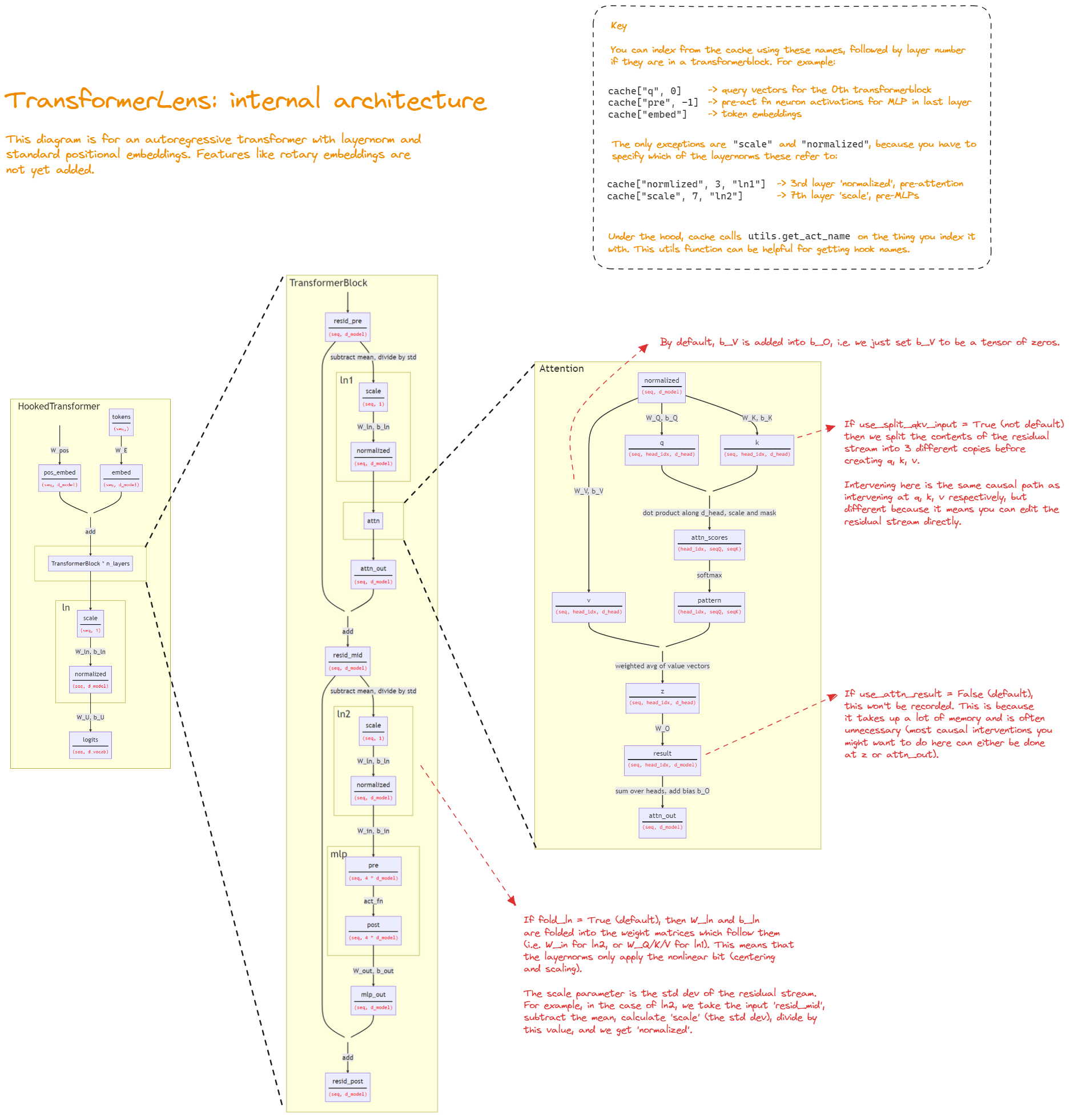
Model overview

ReplacementModel

This module is common for TranscoderSet (set of SingleLayerTranscoders) and CrossLayerTranscoder transcoder architectures

ReplacementModel

  ReplacementModel(
    (embed): Embed()
    (hook_embed): HookPoint()
    (blocks): ModuleList((0-25): 26 x TransformerBlock())  # see `TransformerBlock`
    (ln_final): RMSNorm(
      (hook_scale): HookPoint()
      (hook_normalized): HookPoint()
    )
    (unembed): ReplacementUnembed(
      (old_unembed): Unembed()
      (hook_pre): HookPoint()
      (hook_post): HookPoint()
    )
    (transcoders): ... # see relevant transcoder architecture below (e.g. `TranscoderSet` or `CrossLayerTranscoder`)
  )

• TransformerBlock is a TransformerLens transformer block with additional hooks and a replacement MLP

  TransformerBlock

  (ln1): RMSNorm(
    (hook_scale): HookPoint()
    (hook_normalized): HookPoint()
  )
  (ln1_post): RMSNorm(
    (hook_scale): HookPoint()
    (hook_normalized): HookPoint()
  )
  (ln2): RMSNorm(
    (hook_scale): HookPoint()
    (hook_normalized): HookPoint()
  )
  (ln2_post): RMSNorm(
    (hook_scale): HookPoint()
    (hook_normalized): HookPoint()
  )
  (attn): GroupedQueryAttention(
    (hook_k): HookPoint()
    (hook_q): HookPoint()
    (hook_v): HookPoint()
    (hook_z): HookPoint()
    (hook_attn_scores): HookPoint()
    (hook_pattern): HookPoint()
    (hook_result): HookPoint()
    (hook_rot_k): HookPoint()
    (hook_rot_q): HookPoint()
  )
  (mlp): ReplacementMLP(
    (old_mlp): GatedMLP(
      (hook_pre): HookPoint()
      (hook_pre_linear): HookPoint()
      (hook_post): HookPoint()
    )
    (hook_in): HookPoint()
    (hook_out): HookPoint()
  )
  (hook_attn_in): HookPoint()
  (hook_q_input): HookPoint()
  (hook_k_input): HookPoint()
  (hook_v_input): HookPoint()
  (hook_mlp_in): HookPoint()
  (hook_attn_out): HookPoint()
  (hook_mlp_out): HookPoint(
    (hook_out_grad): HookPoint()
  )
  (hook_resid_pre): HookPoint()
  (hook_resid_mid): HookPoint()
  (hook_resid_post): HookPoint()
  

Transcoders

• When using a TranscoderSet set of SingleLayerTranscoders as the transcoder architecture:

  TranscoderSet

      (transcoders): TranscoderSet(
        (transcoders): ModuleList(
          (0): SingleLayerTranscoder(
            (activation_function): JumpReLU(
              threshold=Parameter containing:
              tensor(0.5664, device='cuda:0', dtype=torch.bfloat16), bandwidth=0.1
            )
          )
          ...
          (25): SingleLayerTranscoder(
            (activation_function): JumpReLU(
              threshold=Parameter containing:
              tensor(6.1250, device='cuda:0', dtype=torch.bfloat16), bandwidth=0.1
            )
          )
        )
      )
  

  
  

• When using a CrossLayerTranscoder as the transcoder architecture:

    (transcoders): CrossLayerTranscoder()
  

  Note on Lazy Decoders

  • lazy_decoders is by default True so to get W_dec (without excessive memory demands) we log W_dec manually from within compute_attribution_components

    {n:p.shape for n,p in model.transcoders.named_parameters()}
    {'W_enc': torch.Size([26, 16384, 2304]), 'b_dec': torch.Size([26, 2304]), 'b_enc': torch.Size([26, 16384])}
    

  • notice since each CLT feature has a single encoder weight but decoder weights that output to each subqeuent layer MLP output, our W_dec are shaped accordingly, n_output_layers = self.n_layers - layer_id

  • the W_dec then is shaped (d_transcoder, n_output_layers, d_model)

  • in addition to lazily loading decoder weights on demand to save memory, only the needed feature ids are loaded as well

    w_dec_shapes = {}
    for l in range(self.n_layers):
        path = os.path.join(self.clt_path, f"W_dec_{l}.safetensors")
        with safe_open(path, framework="pt", device=self.device.type) as f:
            w_dec_shapes[l] = f.get_slice(f"W_dec_{l}")[:].to(device).to(dtype).shape
    print(w_dec_shapes)
    {
    0: torch.Size([16384, 26, 2304]), 
    1: torch.Size([16384, 25, 2304]), 
    ...
    24: torch.Size([16384, 2, 2304]), 
    25: torch.Size([16384, 1, 2304])
    }
    

Precompute Activations, Setup Hooks and Generate AttributionContext

Attribution Hooks Setup and Activation Precomputation

• This phase precomputes the ReplacementModel and transcoder activations as well as the error vectors, saving them and the token embeddings.

    ctx = model.setup_attribution(input_ids)

• get_caching_hooks is used to get mlp in and out caching hooks

          mlp_in_cache, mlp_in_caching_hooks, _ = self.get_caching_hooks(
              lambda name: self.feature_input_hook in name
          ) 
          mlp_out_cache, mlp_out_caching_hooks, _ = self.get_caching_hooks(
              lambda name: self.feature_output_hook in name
          )
  

• get_caching_hooks: normal TL caching hook for getting targeted mlp activations

• run_with_hooks is called with just the mlp in and out caching hooks

  • this collects the original model’s activations and mlp in and out hook points (without using the trained transcoders)

  logits = self.run_with_hooks(tokens, fwd_hooks=mlp_in_caching_hooks + mlp_out_caching_hooks)
  

• Note ReplacementModel when configured adds a hook_out_grad HookPoint to the subblock that handles the skip connection after mlp_out and enables hooking into the gradients of the function (that wouldn’t be possible with backward since the acts are detached)

• the hook_out_grad hook is important as it is the output of the mlp put to the residual (after including the skip connection), used for lots of subsequent computation (error, scores)

  • e.g. when error is calculated below using mlp_out_cache, it uses the special hook_out_grad that was added

Transcoder Architecture-Specific Attribution

• compute_attribution_components is called to collect all attribution_data required for AttributionContext

• this method is transcoder type specific, single layer transcoders form a TranscoderSet that have this method, CrossLayerTranscoders have a different version

    attribution_data = self.transcoders.compute_attribution_components(mlp_in_cache, self.zero_positions)

• we construct the activation_matrix using compute_attribution_components which allows multiple different transcoder architectures to be used

• For TranscoderSet (set of SingleLayerTranscoder)

  TranscoderSet Attribution Context

  
  

  • note that this implementation is for the SingleLayerTranscoders not cross-layer transcoders. CLTs have same number of encoder parameters but num_layers/2 times more decoder parameters and have separate decoder vectors for each subsequent layer. We can see the current reconstruction uses just the corresponding input to that layer and collects that SLT’s output. See the CrossLayerTranscoder version of compute_attribution_components for CLT mechanics

  • we construct per layer sparse activations (zeroing out bos activations also) using our trained transcoders (remember ReplacementMLP is the original model with specially instrumented MLP hooks for inspection/replacement of activations etc)

  • here is where the reconstruction is calculated by passing in the captured/cached mlp_input (mlp_in_cache) to the relevant trained transcoders

  • compute_attribution_components uses encode_sparse and decode_sparse methods on each transcoder layer to collect our required attribution context and package it in a AttributionContext dataclass:

    • activation_matrix: Sparse (n_layers, n_pos, d_transcoder) activations

    • reconstruction: (n_layers, n_pos, d_model) reconstructed outputs

    • encoder_vecs: Concatenated encoder vectors for active features

    • decoder_vecs: Concatenated decoder vectors (scaled by activations)

    • encoder_to_decoder_map: Mapping from encoder to decoder indices

    • encode_sparse

      • accepts incoming activations (for SLT, feature_input_hook is ln2.hook_normalized) and uses the current layer’s self.W_enc and b_enc to calc pre_acts and the activation function to calc the acts, sets the bos acts to 0 and calculates the active (nnz, indices()) encoders

      • these are the local replacement model transcoder preactivations

      • gets non-zero indices, getting the trained transcoder encoder layers (transposed) for active features

      • NOTE: crucially, these target transcoder feature preactivations are linear in each upstream source transcoder feature activations since we freeze attention patterns and normalization denominators!

      • example sparse_acts, active_encoder shapes for gemma layer 0:

      sparse_acts.shape  
      torch.Size([9, 16384])  # n_pos, d_transcoder
      active_encoders.shape
      torch.Size([634, 2304]) # num_active_features for the layer, d_model
      

    • decode_sparse

      • accepts the decoded output activations and scales the relevant W_dec indices by the activations

      • Return decoder rows for active features only from the trained transcoders

      • uses indices() to get non-zero indices so requires sparse tensor

      • for each active feature index for each layer, creates a [n_active_features_for_layer, d_model] tensor

      • example shapes for gemma layer 0

        W_dec.shape
        torch.Size([16384, 2304])
        transcoders[layer].W_dec[feat_idx].shape
        torch.Size([634, 2304])
        

  
  

• For CrossLayerTranscoder Attribution Context

  CrossLayerTranscoder Attribution Context

  
  

  • a crucial difference between SLT and CLT attribution flows is that for SLT, decode_sparse returns a per-layer reconstruction, whereas for CLT, a separate compute_reconstruction step is required to calculate and store the reconstruction separately for each subsequent layer it outputs to (since each layer has a separate decoder for each subsequent layer)

  • encode_sparse

      sparse_acts, active_encoders = transcoder.encode_sparse(mlp_inputs[layer], zero_first_pos=True)
  

  • select_decoder_vectors

          pos_ids, layer_ids, feat_ids, decoder_vectors, encoder_to_decoder_map = (
              self.select_decoder_vectors(features)
      )
  

  • compute_reconstruction

      reconstruction = self.compute_reconstruction(pos_ids, layer_ids, decoder_vectors)    
  

Analysis Point Data: See below sampled data for the current attribution example at the end of Transcoder-Specific attribution described above.

Show code cell source

Hide code cell source

analysis_injector.get_output("ap_compute_attribution_end")

Key	Inspected Output	Annotation
attribution_data['reconstruction'].shape	(26, 9, 2304)	n_layers, n_pos, d_model
attribution_data['decoder_vecs'].shape	(7140, 2304)	num_active_features, d_model

Error Vectors and Reconstruction

• Finally, we then compute the error vectors, the actual (replacement)MLP layers, the mlp_out_cache are the original acts and the reconstructed-from transcoder acts are the reconstruction

  error_vectors = mlp_out_cache - attribution_data["reconstruction"]
  

• we also save the token vector positions

  token_vectors = self.W_E[tokens].detach()  # (n_pos, d_model)
  

• all the per-layer active feature decoder vectors are scaled by how much each transcoder feature was activated

• at the end of setup_attribution we, package the attribution components into an AttributionContext

Analysis Point Data: See below sampled data for the current attribution example at the end of Precompute Activations, Setup Hooks and Generate AttributionContext.

Show code cell source

Hide code cell source

analysis_injector.get_output("ap_setup_attribution_end")

Key	Inspected Output	Annotation
ctx.activation_matrix.shape	(26, 9, 16384)
ctx.decoder_vecs.shape	(7140, 2304)
ctx.encoder_vecs.shape	(7140, 2304)
ctx.logits.shape	(1, 9, 256000)
ctx.token_vectors.shape	(9, 2304)
ctx.error_vectors.shape	(26, 9, 2304)
ctx.encoder_to_decoder_map.shape	(7140,)
ctx.decoder_locations.shape	(2, 7140)
n_layers	26
_row_size	7383	total_active_feats + error_nodes ((n_layers + 1) * n_pos) # + logits later

Show code cell source

Hide code cell source

analysis_injector.get_output("ap_precomputation_phase_end")

Key	Value
target_token_ids	[26865, 22605]
target_logits	[23.375, 25.75]
target_tokens	['▁Dallas', '▁Austin']

Forward Pass

• When we run the forward pass, we do so under the install_hooks context manager of the AttributionContext object we created above:

      def install_hooks(self, model: "ReplacementModel"):
          """Context manager instruments the hooks for the forward and backward passes."""
          with model.hooks(
              fwd_hooks=self._caching_hooks(model.feature_input_hook),  # type: ignore
              bwd_hooks=self._make_attribution_hooks(model.feature_output_hook),  # type: ignore
          ):
              yield
  

• AttributionContext._caching_hooks fwd hooks are installed

  • these cache the layerwise residual activations for the replacement model in AttributionContext._resid_activations (as well as the unembed.hook_pre acts after the last layer)

  • for this gemma example, the hook currently used for SLT is the feature_input_hook ln2.hook_normalized and for CLT hook_resid_mid (so the input for the MLP/transcoder)

• AttributionContext._make_attribution_hooks bwd hooks are installed

  • these are the bwd hooks installed below via _make_attribution_hooks

  • a model.forward is run (stopping at the last layer), note the input is expanded to the batch_size num of nodes to process per position, so with context size 9 and a batch_size of 256 for this example, our input would be torch.Size([256, 9])

  • the final residual activations are set on the context manager ctx._resid_activations[-1] = model.ln_final(residual)

  • after the forward, the ReplacementModel MLP block modules can be offloaded (all original module MLP blocks [block.mlp for block in model.blocks])

Key Bwd Hooks: _make_attribution_hooks

• _make_attribution_hooks is a function that associates the bwd attribution hook factory function _compute_score_hook with the feature/logit, error and token node types. Inside the TransformerLens hooks context manager, these hooks are enabled and installed during the forward pass in this phase (phase 1)

• These hooks are subsequently used for both logit attribution (Phase 3) and feature attribution (Phase 4)

  • for phase 3, the gradient of the pre-softmax logit (minus the mean logit) is injected as the demeaned logits are passed to compute_batch and backward is run while injecting the relevant gradients to einsum with the source decoder vectors

  • for phase 4, the upstream target encoder vectors are similarly injected (see key attribution gradient flow summary below)

  • see compute_batch below for the mechanics of using backward hooks to orchestrate logit/feature/error/token node attribution

• Attribution Hook Details

  Node Attribution Hook Construction

  
  

  • the feature/logit node attribution bwd hooks are constructed:

    1. layerwise using active features (non-zero activations) from the precomputed activation_matrix sparse indices

       nnz_layers, nnz_positions = self.decoder_locations
       

       • nnz_layers, nnz_positions are the non-zero indices for layers and positions dimensions of activation_matrix.indices()

       • for this gemma example, layer 25 has 265 active features distributed across all 8 positions (position 0 is bos so is zeroed out), e.g. 31 features active at position 8:

         nnz_layers[-265:].unique()
         tensor([25], device='cuda:0')
         nnz_positions[-265:].unique()
         tensor([1, 2, 3, 4, 5, 6, 7, 8], device='cuda:0')
         nnz_positions[-31:].unique()
         tensor([8], device='cuda:0')
         

    2. by passing in the appropriate feature decoder vectors (from the trained transcoders)

       # Feature nodes
       feature_hooks = [
           self._compute_score_hook(
               f"blocks.{layer}.{feature_output_hook}",
               self.decoder_vecs[layer_mask],
               write_index=self.encoder_to_decoder_map[layer_mask],  # type: ignore
               read_index=np.s_[:, nnz_positions[layer_mask]],  # type: ignore
           )
           for layer in range(n_layers)
           if (layer_mask := nnz_layers == layer).any()
       ]
       

    • The np.s_ indexing functionality is used to construct a slice that can be used to select the appropriate “gradient” vectors from the injected logit_vecs in our backward pass.

      • All rows in the first dimension (the batch dimension, in this case our logit_vecs batch where only 10 of the 256 rows will be active) are selected.

      • For the second dim, the residual activation position indices that are associated with non-zero feature activations in our activation_matrix for each layer.

    • This will result in the appropriate logit_vec “grads” vectors getting selected repeatedly for the appropriate positions that have active features for that layer.

    • Concretely, for layer 25 in our gemma SLT example, we see the logit_vec injected “grads” we einsum with our output_vecs decoder_vecs slice (265 active decoder vecs associated with features for that layer) for the given layer results in the desired shapes for our einsum. Each target logit_vec will be repeated 31 times for position 8 so the corresponding 31 active feature decoder vectors for position 8 will be einsum’d with them and written to the appropriate positions in our attribution score tensor:

      # these are the pos indices associated with the active features for layer 25
      read_index[1]
      tensor([1, 1, 1, 1, 1, 1, 1, 1, 1, 1, 1, 1, 1, 1, 1, 1, 1, 1, 1, 1, 1, 1, 1, 1,
              1, 1, 1, 1, 1, 1, 1, 1, 1, 1, 1, 1, 1, 1, 1, 1, 1, 1, 1, 1, 1, 1, 1, 1,
              1, 1, 1, 1, 1, 1, 1, 1, 1, 1, 1, 1, 1, 1, 1, 1, 1, 1, 1, 1, 1, 1, 1, 2,
              2, 2, 2, 2, 2, 2, 2, 2, 2, 2, 2, 2, 2, 2, 2, 2, 2, 2, 2, 2, 2, 2, 2, 2,
              2, 2, 2, 2, 2, 2, 2, 2, 2, 2, 2, 3, 3, 3, 3, 3, 3, 3, 3, 3, 3, 3, 3, 3,
              3, 3, 3, 3, 3, 3, 3, 3, 3, 3, 3, 4, 4, 4, 4, 4, 4, 4, 4, 4, 4, 4, 4, 4,
              4, 4, 4, 4, 4, 4, 4, 4, 4, 4, 4, 4, 4, 4, 4, 5, 5, 5, 5, 5, 5, 5, 5, 5,
              5, 5, 5, 5, 5, 5, 5, 5, 5, 5, 5, 5, 5, 5, 5, 5, 5, 5, 5, 5, 5, 5, 5, 5,
              5, 6, 6, 6, 6, 6, 6, 6, 6, 6, 6, 6, 6, 6, 6, 6, 6, 6, 6, 6, 6, 6, 6, 7,
              7, 7, 7, 7, 7, 7, 7, 7, 7, 7, 7, 7, 7, 7, 7, 7, 7, 7, 8, 8, 8, 8, 8, 8,
              8, 8, 8, 8, 8, 8, 8, 8, 8, 8, 8, 8, 8, 8, 8, 8, 8, 8, 8, 8, 8, 8, 8, 8,
              8], device='cuda:0')
      read_index[1].shape
      torch.Size([265])
      
      write_index.shape  # corresponding active feature decoder vec indices
      torch.Size([265])
      write_index.min()
      tensor(6850, device='cuda:0')
      write_index.max()
      tensor(7114, device='cuda:0')
      
      grads.shape
      torch.Size([256, 9, 2304])  # batch_size, n_pos, d_model
      grads.to(output_vecs.dtype)[read_index].shape
      torch.Size([256, 265, 2304])  # batch_size, num active position/feature combos for layer, d_model
      
      output_vecs.shape
      torch.Size([265, 2304])  # num active position/feature combos for layer, d_model
      

  • the error and token node hooks are constructed similarly, except:

    1. an error_offset function is used to calculate the appropriate node indices

       def error_offset(layer: int) -> int:  # starting row for this layer
           return self.activation_matrix._nnz() + layer * n_pos
       

    2. instead of binding the scaled decoder vectors to the hooks, the error and token node hooks use the precomputed error_vectors and token_vectors respectively”

       error_hooks = [
           self._compute_score_hook(
               f"blocks.{layer}.{feature_output_hook}",
               self.error_vectors[layer],
               write_index=np.s_[error_offset(layer) : error_offset(layer + 1)],
           )
           for layer in range(n_layers)
       ]
       
       # Token-embedding nodes
       tok_start = error_offset(n_layers)
       token_hook = [
           self._compute_score_hook(
               "hook_embed",
               self.token_vectors,
               write_index=np.s_[tok_start : tok_start + n_pos],
           )
       ]
       

  • The actual bwd hook binds our AttributionContext ref to form the closure we use to output the attribution scores to the correct rows in our attribution score edge matrix. The scores are buffered on a per-batch basis, each batch calculating the source attribution scores for all nodes w.r.t. the current batch size of target nodes:

        def _compute_score_hook(
            self,
            hook_name: str,
            output_vecs: torch.Tensor,
            write_index: slice,
            read_index: slice | np.ndarray = np.s_[:],
        ) -> tuple[str, Callable]:
            """
            Factory that contracts *gradients* with an **output vector set**.
            The hook computes A_{s->t} and writes the result into an in-place buffer row.
            """
    
            proxy = weakref.proxy(self)
    
            def _hook_fn(grads: torch.Tensor, hook: HookPoint) -> None:
                proxy._batch_buffer[write_index] += einsum(
                    grads.to(output_vecs.dtype)[read_index],
                    output_vecs,
                    "batch position d_model, position d_model -> position batch",
                )
    
            return hook_name, _hook_fn
    

Analysis Point Data: See below sampled data for the current attribution example at the end of Forward Pass.

Show code cell source

Hide code cell source

analysis_injector.get_output("ap_forward_pass_end")

Key	Value
target_token_ids	[26865, 22605]
target_logits	[31.125, 39.0]
target_tokens	['▁Dallas', '▁Austin']

Build Input Vectors

We filter active features of our cached transcoder activation_matrix and depending on our target logits mode, generate our feature matrices we want to use in subsequent analysis by using either the:

1. configured cumulative probability and max_n_logits if in the baseline default compute_salient_logits target logits mode

2. specific logits specified by token id or token if we use our compute_specific_logits target logits mode

Analysis Point Data: See below sampled data for the current attribution example at the end of Build Input Vectors.

Show code cell source

Hide code cell source

analysis_injector.get_output("ap_build_input_vectors_end")

Key	Inspected Output	Annotation
logit_idx	[22605, 573, 235248, 9778, 9447, 235292, 26865, 476, 3151, 109]
logit_p	[0.304688, 0.126953, 0.077148, 0.046875, 0.04126, 0.032227, 0.028442, 0.028442, 0.022095, 0.017212]	logit probabilities
target_tokens	['▁Austin', '▁Dallas']
target_logit_indices	[0, 6]
target_logit_p	[0.304688, 0.028442]
logit_cumulative_prob	0.7265625
total_nodes	7393
max_feature_nodes	7140
total_active_feats	7140
n_logits	10
n_layers	26
n_pos	9
max_n_logits	10
edge_matrix.shape	torch.Size([7150, 7393])
row_to_node_index.shape	torch.Size([7150])
logit_vecs.shape	torch.Size([10, 2304])

Core compute_batch Attribution Logic

In the Compute Logit Attributions and Compute Feature Attributions phases, it’s important to note we aren’t using conventional gradient propagation but rather using backward() as a convenient orchestration mechanism to calculate our desired node attributions via custom gradient injection.

The core mechanics of this are:

1. The compute_batch method of AttributionContext which is shared among both the Logit and Feature Node Attribution phases:

   Snapshot of `compute_batch`

   
   

       def compute_batch(
           self,
           layers: torch.Tensor,
           positions: torch.Tensor,
           inject_values: torch.Tensor,
           retain_graph: bool = True,
       ) -> torch.Tensor:
           """Return attribution rows for a batch of (layer, pos) nodes.
   
           The routine overrides gradients at **exact** residual-stream locations
           triggers one backward pass, and copies the rows from the internal buffer.
   
           Args:
               layers: 1-D tensor of layer indices *l* for the source nodes.
               positions: 1-D tensor of token positions *c* for the source nodes.
               inject_values: `(batch, d_model)` tensor with outer product
                   a_s * W^(enc/dec) to inject as custom gradient.
   
           Returns:
               torch.Tensor: ``(batch, row_size)`` matrix - one row per node.
           """
   
           assert self._resid_activations[0] is not None, "Residual activations are not cached"
           batch_size = self._resid_activations[0].shape[0]
           self._batch_buffer = torch.zeros(
               self._row_size,
               batch_size,
               dtype=inject_values.dtype,
               device=inject_values.device,
           )
   
           # Custom gradient injection (per-layer registration)
           batch_idx = torch.arange(len(layers), device=layers.device)
   
           def _inject(grads, *, batch_indices, pos_indices, values):
               grads_out = grads.clone().to(values.dtype)
               grads_out.index_put_((batch_indices, pos_indices), values)
               return grads_out.to(grads.dtype)
   
           handles = []
           layers_in_batch = layers.unique().tolist()
   
           for layer in layers_in_batch:
               mask = layers == layer
               if not mask.any():
                   continue
               fn = partial(
                   _inject,
                   batch_indices=batch_idx[mask],
                   pos_indices=positions[mask],
                   values=inject_values[mask],
               )
               resid_activations = self._resid_activations[int(layer)]
               assert resid_activations is not None, "Residual activations are not cached"
               handles.append(resid_activations.register_hook(fn))
   
           try:
               last_layer = max(layers_in_batch)
               self._resid_activations[last_layer].backward(
                   gradient=torch.zeros_like(self._resid_activations[last_layer]),
                   retain_graph=retain_graph,
               )
           finally:
               for h in handles:
                   h.remove()
   
           buf, self._batch_buffer = self._batch_buffer, None
           return buf.T[: len(layers)]
   

   
   

2. Logit and Feature Attribution-Specific invocations of compute_batch

   Logit Attribution Computation

   
   

       for i in range(0, len(logit_idx), batch_size):
           batch = logit_vecs[i : i + batch_size]
           rows = ctx.compute_batch(
               layers=torch.full((batch.shape[0],), n_layers),
               positions=torch.full((batch.shape[0],), n_pos - 1),
               inject_values=batch,
           )
           edge_matrix[i : i + batch.shape[0], :logit_offset] = rows.cpu()
           row_to_node_index[i : i + batch.shape[0]] = (
               torch.arange(i, i + batch.shape[0]) + logit_offset
           )
   

   
   
   Feature Attribution Computation

   
   

   queue = [pending[i : i + batch_size] for i in range(0, len(pending), batch_size)]
   
   for idx_batch in queue:
       n_visited += len(idx_batch)
   
       rows = ctx.compute_batch(
           layers=feat_layers[idx_batch],
           positions=feat_pos[idx_batch],
           inject_values=ctx.encoder_vecs[idx_batch],
           retain_graph=n_visited < max_feature_nodes,
       )
   
       end = min(st + batch_size, st + rows.shape[0])
       edge_matrix[st:end, :logit_offset] = rows.cpu()
       row_to_node_index[st:end] = idx_batch
       visited[idx_batch] = True
       st = end
       pbar.update(len(idx_batch))
   

Key Attribution Flow Summary

The _compute_score_hook invoked by compute_batch as described below will calculate the tensor product of:

1. the the unembed vectors (for target logit node attribution) or the relevant target layer encoder vecs (for target feature node attribution)

2. and (for feature nodes) the relevant layer’s activation-scaled transcoder decoder vectors (which represent the feature space transformation).

This allows us to score how much each feature (scaled by activation) contributes to the residual stream in the unembed (for logit attribution) or target transcoder encoder vec feature (for feature-feature attribution) vector’s direction

Compute Logit Attributions

Remembering our score computation hooks were registered layer-wise with individual per-layer hook registration, our custom gradient injection hooks are similarly registered layer-wise in compute_batch

In the case of the gemma SLT example with max_n_logits = 10, we only have 1 set of resid_activations (from layer 26) to register our hooks for since we’re computing source node attributions for all nodes w.r.t. only the 10 logit_vecs (logit_vecs.shape = max_n_logits, d_model), so layers_in_batch = [26]

• concretely:

  batch.shape
  torch.Size([10, 2304])
  logit_vecs.shape
  torch.Size([10, 2304])
  (layer, len(inject_values[mask]), batch_idx[mask], positions[mask])
  (26, 10, tensor([0, 1, 2, 3, 4, 5, 6, 7, 8, 9]), tensor([8, 8, 8, 8, 8, 8, 8, 8, 8, 8])) 
  

• each batch will only have non-zero entries in the first 10 rows of dim 0:

  has_nonzero = torch.any(grads.to(output_vecs.dtype)[read_index] != 0, dim=(1, 2))
  nz_indices = torch.where(has_nonzero)[0]
  nz_indices
  tensor([0, 1, 2, 3, 4, 5, 6, 7, 8, 9], device='cuda:0')
  

We register a backward hook for the last layer (layer 26 in this case) ctx._resid_activations[int(layer)] that injects our custom logit_vecs (demeaned and transposed logit unembed col vectors) as gradient.

For each batch, as backward() is executed the relevant layer-wise hooks are triggered filling in the corresponding rows of our attribution score buffer layer-by-layer via the einsum in our _compute_score_hook bwd hook. The number of elements filled per-hook correspond to the per-layer number of active nodes (feature, error or token):

def _compute_score_hook(
# ...

    proxy = weakref.proxy(self)

    def _hook_fn(grads: torch.Tensor, hook: HookPoint) -> None:
        proxy._batch_buffer[write_index] += einsum(
            grads.to(output_vecs.dtype)[read_index],
            output_vecs,
            "batch position d_model, position d_model -> position batch",
        )
    return hook_name, _hook_fn

Note we always retain_graph for these backward hooks for subsequent use. compute_batch then returns the batch buffer (which is simultaneously zeroed out on the object) which includes the feature nodes + error nodes + token nodes attributions for each of the logits (as rows)

The edge matrix is then updated using the calculated node attributions in rows (while leaving the last max_n_logit (10) logit entries 0), so the first 10 rows in edge_matrix are populated except for the last 10 columns, the remaining elements are all zero at this point since we’re just building the logit attribution entries.

We finally update the row_to_node_index with the logit node mapping, so in this case, logit rows 0:10 map to the last 10 edge_matrix columns, while the 11th flattened node is the first feature node and doesn’t have a mapping yet.

Reproducing A Specific Node Attribution Calculation

• Let’s inspect the attribution of a specific node (e.g. 6334), to make this concrete. We can set a break in our custom bwd hook and validate the calculation written to our buffer for the target index 6334. This is the einsum referenced above:

  proxy._batch_buffer[write_index] += einsum(grads.to(output_vecs.dtype)[read_index], output_vecs,
      "batch position d_model, position d_model -> position batch",
  )
  

• The relevant shapes of the tensors involved in this calculation are:

  grads.to(output_vecs.dtype)[read_index].shape # logit_vecs (demeaned and transposed unembedding vectors)
  torch.Size([256, 81, 2304])  # batch_size, layer 20 active nodes, d_model
  output_vecs.shape  # active decoder_vecs for layer
  torch.Size([81, 2304])       # layer 20 active nodes, d_model
  write_index.shape
  torch.Size([81]) # layer 20 active nodes
  read_index[1].shape
  torch.Size([81]) # layer 20 active nodes
  

• In this case, we only run compute_batch one time since we have fewer than 256 target nodes we want to calculate source attribution scores for. Since we’re using backward() for orchestration, we only need to trigger a single backward() that processes all layer-wise score hooks as appropriate for our source nodes. The write_index writes to our score buffer which for each batch (again, just 1 in this case) is of shape (n_logits, logit_offset)

• All feature, error and token node scores are calculated, we show just the feature_hooks below. The returned rows for each logit computation batch (just 1) is shape (10, 7358) in this case because we have 10 target logits and 7358 total source nodes (feature, error and token nodes).

• We isolate the relevant indices for our target node 6334, we only have 10 nodes in this batch since we’re only calculating source attributions for the 10 target logit nodes.:

  target_node_id = 6334
  target_buf_index = torch.where(write_index == target_node_id)
  orig_grad_slice = grads.to(output_vecs.dtype)[read_index].detach()
  grads_slice = orig_grad_slice[:10, target_buf_index, :].squeeze()
  output_vecs_slice = output_vecs[target_buf_index].squeeze()
  (grads_slice.shape, output_vecs_slice.shape)
  (torch.Size([10, 2304]), torch.Size([2304]))
  

• We can then reproduce the einsum calculation directly to validate the attribution for our target node 6334

  torch.matmul(grads_slice, output_vecs_slice)
  tensor([ 6.5625e+00, -1.4258e-01, -2.7344e-02,  8.3750e+00,  2.7656e+00,
          -2.0020e-01, -6.8359e-03,  6.0312e+00, -2.2339e-02,  2.8931e-02],
      device='cuda:0', dtype=torch.bfloat16)
  

• So what are the attributions to our feature node 6334 for our target_logit_indices?

  • We projected our decoder vector (associated with node 6334) into the unembed vec direction for each of our top logits individually.

  • For our target token (’▁Austin’, ‘▁Dallas’) logit indexes, elements 0 and 7, we see 6.5625 and 6.0312.

  • As expected, our initial attribution for active feature index 6334 after compute logit attribution:

    • returned buffer:

    buf.T[:10][[0,7], 6334]  # returned buffer from `compute_batch`
    tensor([6.5625, 6.0312], device='cuda:0', dtype=torch.bfloat16)
    edge_matrix[[0, 7], 6334]  # logit nodes are initially the first `max_n_logits` target nodes
    tensor([6.5625, 6.0312])
    

Attribution Node Id to (Graph) Feature Id Mapping

• If you want to associate these internal node attributions to feature ids on our attribution graphs, we need to map the node ids back to feature ids (we have helper functions for this but it’s good to understand the mechanics)

• remember the ctx.activation_matrix saves non-zero activations by feature_idx (0:d_transcoder) for each layer for each position:

        ctx.activation_matrix
        tensor(indices=tensor([[    0,     0,     0,  ...,    25,    25,    25],
                        [    1,     1,     1,  ...,     8,     8,     8],
                        [   41,    96,   253,  ..., 16014, 16302, 16326]]),
        values=tensor([ 2.5156,  3.5312,  0.7070,  ...,  7.4375, 40.7500,
                        12.2500]),
        device='cuda:0', size=(26, 9, 16384), nnz=7115, dtype=torch.bfloat16,
        layout=torch.sparse_coo)

• the encoder_to_decoder_map map is just a vector activation_matrix._nnz long (for SLT) that can be used to associate active encoder and decoder vecs to the activation matrix.

• for example for layer 20, find the positions in our activation_matrix._nnz length vector of active decoders

        per_layer_mask = (nnz_layers == 20)
        nnz_positions[per_layer_mask]
        tensor([1, 1, 1, 1, 1, 1, 2, 2, 2, 2, 2, 2, 2, 2, 2, 3, 3, 3, 3, 3, 3, 3, 3, 3,
                3, 4, 4, 4, 4, 4, 4, 4, 4, 4, 4, 4, 5, 5, 5, 5, 5, 5, 5, 5, 5, 5, 5, 5,
                6, 6, 6, 6, 6, 6, 6, 6, 6, 7, 7, 7, 7, 7, 7, 7, 7, 7, 7, 7, 7, 8, 8, 8,
                8, 8, 8, 8, 8, 8, 8, 8, 8], device='cuda:0')

• so our active decoders for layer 20 are

        ctx.decoder_vecs[per_layer_mask].shape
        torch.Size([81, 2304])

• and the appropriate activation_matrix indices using encoder_to_decoder_map

        ctx.encoder_to_decoder_map[per_layer_mask]
        tensor([6254, 6255, 6256, 6257, 6258, 6259, 6260, 6261, 6262, 6263, 6264, 6265,
                6266, 6267, 6268, 6269, 6270, 6271, 6272, 6273, 6274, 6275, 6276, 6277,
                6278, 6279, 6280, 6281, 6282, 6283, 6284, 6285, 6286, 6287, 6288, 6289,
                6290, 6291, 6292, 6293, 6294, 6295, 6296, 6297, 6298, 6299, 6300, 6301,
                6302, 6303, 6304, 6305, 6306, 6307, 6308, 6309, 6310, 6311, 6312, 6313,
                6314, 6315, 6316, 6317, 6318, 6319, 6320, 6321, 6322, 6323, 6324, 6325,
                6326, 6327, 6328, 6329, 6330, 6331, 6332, 6333, 6334], device='cuda:0')

• for the our example feature we’re probing in ctx.encoder_to_decoder_map, what is the active feature index that we got our active encoder and decoder vecs from in activation_matrix?

        ctx.activation_matrix.indices().T[6334]
        tensor([   20,     8, 15589], device='cuda:0')

• so layer 20, position 8, feature id 15589 is the feature that corresponds to node id 6334

• using activation_matrix directly to probe all features active at layer 20, position 8 and their corresponding values, we see we can expect feature 15589 to have an activation of 52.0 in our graph UI

        active_indices = ctx.activation_matrix.indices()
        test_mask = (active_indices[0] == 20) & (active_indices[1] == 8)
        filtered_indices = active_indices[:, test_mask]
        filtered_values = ctx.activation_matrix.values()[test_mask]

        filtered_indices.T
        tensor([[   20,     8,   114],
                [   20,     8,   438],
                [   20,     8,  3094],
                [   20,     8,  5433],
                [   20,     8,  5916],
                [   20,     8,  6026],
                [   20,     8, 10118],
                [   20,     8, 10254],
                [   20,     8, 15133],
                [   20,     8, 15276],
                [   20,     8, 15366],
                [   20,     8, 15589]], device='cuda:0')
        filtered_values
        tensor([15.5625,  7.8125, 16.7500,  7.5312, 45.7500, 14.8750, 12.1875, 19.0000,
                8.0000, 14.4375,  7.2812, 52.0000], device='cuda:0',
        dtype=torch.bfloat16)

Analysis Point Data: See below sampled data for the current attribution example at the end of Compute Logit Attributions.

analysis_injector.get_output("ap_compute_logit_attribution_end")

Key	Inspected Output	Annotation
edge_matrix.shape	(7150, 7393)
row_to_node_index.shape	(7150,)
logit_section.shape	torch.Size([10, 7140])
logit_section_zeros_info	(torch.Size([216]), 6895, 7110)	logit section zeros shape, min node id, max node id
logit_section_zero_feature_range	6894: (24, 8, 16258) 6895: (25, 1, 209) 7110: (25, 7, 15301) 7111: (25, 8, 553)	In the final layer, only the final position has non-zero feature attributions.

Compute Feature Attributions

• Note that the edge_matrix (adjacency matrix) analyzed below is indexed as (target, source) (targets are rows)

• When the graph is pruned, source input edges are normalized for each source node so that they sum to 1 for each target.

• if we are operating on all features (since our max_feature_nodes has been set to equal our total_active_feats) we can run compute_batch below on all the features

• if we are only operating on a subset of features, we first have to run compute_partial_influences to sort all the features by logit influence and then score only those features

• compute_batch is run once per batch (256 in this example) of nodes to analyze, similar to logit attribution above but instead of injecting logit_vecs, we inject the relevant target feature (transcoder encoder vecs) as the gradient.

• Also, instead of just a single compute_batch (with only 10 of the 256 rows populated) and a single backward call, we have many more batches to process that will be fully populated (except for the last batch)

  • e.g., for this gemma SLT example, we need to compute the source influence vectors for all target active features (7115) which requires 28 batches of 256 nodes each (the last batch will only have 203 nodes)

    len(queue)
    28
    

• Our node source vectors are the same as described in logits attribution above (ctx bound in the first forward pass) but we einsum the injected target encoder_vecs with them in our bwd hooks to calculate the feature-to-feature attributions

• each batch involves registering the relevant cached resid activations for the layers in a given batch (a batch can cross layer boundaries)

• the max layer in the batch then has backward() called which allows us to calculate the matmul of the scaled decoder vec for each active feature (or the token_vecs for the token_vec range, which is the case for layer 0 encoders) with the injected target encoder_vecs for active features.

• Another non-feature case are attribution hooks where the output_vecs are the error_vectors (n_layers, n_pos, d_model), playing the same role as the scaled decoder vecs do in the feature node attributions

• we retain_graph for as long as we have another batch to compute

• we queue up update_interval (default 4) * batch_size (so 1024 in this example) nodes unless we have fewer than that left to process

Post-Attribution Edge Matrix

• edge_matrix inspection after feature attributions but before reshaping to full_edge_matrix (so first 10 rows are still logit nodes)

• at this point we have non-normalized influence scores for all logit/feature feature/feature edges so the target vectors are pretty dense:

        edge_matrix[0, :].count_nonzero()
        tensor(7091)
        edge_matrix[6344, :].count_nonzero()
        tensor(6423)

• An error node exists for every token for every layer. We also have the token nodes themselves.

# n_error_nodes = (num_layers + 1) * num_tokens = num_layers * num_tokens + num_tokens

• for the gemma SLT example, edge_matrix at this point is shaped as (7125, 7368):

# n_logits(10) + n_feature_nodes(7115) -> 7125
# n_feature_nodes(7115) + n_error_nodes(234) + n_tokens(9) + n_logits(10) -> 7368

Analysis Point Data: See below sampled data for the current attribution example at the end of Compute Feature Attributions.

analysis_injector.get_output("ap_compute_feature_attributions_end")

Key	Inspected Output	Annotation
target_tokens	['▁Austin', '▁Dallas']
target_logit_p	[0.304688, 0.028442]
top_init_edge_indices	[6390, 7381, 7364, 6462, 6695] [7381, 6390, 6462, 6067, 5952]
top_init_edge_features	{6390: (20, 8, 15589), 6462: (21, 8, 5943), 6695: (23, 8, 12237), 7364: 'non-feature node', 7381: 'non-feature node'} {5952: (14, 7, 2268), 6067: (16, 7, 25), 6390: (20, 8, 15589), 6462: (21, 8, 5943), 7381: 'non-feature node'}
top_init_edge_vals	[6.5625, 6.1875, 3.96875, 3.546875, 2.84375] [10.0625, 6.0625, 3.921875, 3.15625, 2.96875]
features_processed	7140
max_features	7140
progress	100.0%
edge_matrix.shape	(7150, 7393)	( (n_logits + n_feature_nodes), n_feature_nodes + n_error_nodes + n_token_nodes + n_logits

Graph Packaging

Before packaging the our attribution matrices into a circuit-tracer Graph object, note our top influencing features are not the same as the raw activations you’ll see in the graph from activation_matrix. They are our computed feature influences (depending on context, normalized or not-yet-normalized)

In our analysis point below you can see our top inspected token first order and second order feature attributions.

• Note this is not yet converted to abs values and normalized so that the input edges sum to 1. The target logit attribution sums do not correspond directly to logit probs but are rather the non-normalized influence scores

• We refer to the top influencing nodes of the top nodes influencing our inspected logits as per token pre_prune_2nd_order matrices.

• Our helper functions mask out the error and token nodes from these 2nd order influence matrices since by definition those nodes won’t have input feature nodes.

Prior to graph packaging, we reshape our edge_matrix to have the logit nodes at the end and use it to populate the input full_edge_matrix which will be passed to the Graph constructor as our initial (pre-pruned) adjacency matrix.

Our adjacency matrix will have the following shape (n_total_nodes, n_total_nodes). Where n_total_nodes is:

n_feature_nodes + n_error_nodes + n_token_nodes + n_logits

Analysis Point Data: See below sampled data for the current attribution example prior to Graph Packaging.

analysis_injector.get_output("ap_graph_creation_start")

Key	Inspected Output	Annotation
full_edge_matrix.shape	(7393, 7393)
edge_matrix.shape	(7150, 7393)
pre_normalized_logit_node_sum	[33.383419, 28.747423]	Sum of all source nodes for our target logits before normalization
n_total_nodes	7393	len(selected_features):(n_layers * n_pos):n_pos:n_logits
pre_prune_1st_order_idxs	'▁Austin': [6390, 7381, 7364, 6462, 6695] '▁Dallas': [7381, 6390, 6462, 6067, 5952]
pre_prune_1st_order_vals	'▁Austin': [6.5625, 6.1875, 3.9688, 3.5469, 2.8438] '▁Dallas': [10.0625, 6.0625, 3.9219, 3.1562, 2.9688]
pre_prune_2nd_order_idxs	'▁Austin': [7381, 5952, 6067, 2218, 6249] [3, 4, 1, 0, 2] [3, 4, 1, 0, 2] [6247, 7292, 6074, 7310, 6316] [6462, 7381, 6390, 6552, 6314] '▁Dallas': [3, 4, 1, 0, 2] [7381, 5952, 6067, 2218, 6249] [6247, 7292, 6074, 7310, 6316] [7381, 5952, 4230, 2218, 7282] [7381, 4230, 2218, 7228, 7377]
pre_prune_2nd_order_vals	'▁Austin': [51.25, 17.125, 15.0625, 10.625, 10.25] [-inf, -inf, -inf, -inf, -inf] [-inf, -inf, -inf, -inf, -inf] [13.0, 9.0625, 9.0, 6.875, 6.6875] [10.9375, 7.875, 6.9062, 5.9062, 5.2812] '▁Dallas': [-inf, -inf, -inf, -inf, -inf] [51.25, 17.125, 15.0625, 10.625, 10.25] [13.0, 9.0625, 9.0, 6.875, 6.6875] [29.375, 22.25, 10.8125, 6.5, 5.0625] [27.0, 7.5, 5.875, 1.2656, 1.0781]

Graph Pruning, Creation and Saving

Prune by Node/Edge Influence

We next inspect graph pruning process prune_graph following the transformation of our target logits raw target (logit) node attribution through the compute_node_influence and compute_edge_influence functions.

The first step to computing our node influences is to normalize our adjacency matrix above. We then use this normalized adjacency matrix to compute node influences influence via a numerical approach to Neumann series calculation.

Iterative computing of our node influence vector starts with seeding our logit_weights via our direct logit probabilities. We then multiply those weights with our adjacency matrix logit_weights @ A to construct the initial current_influence vector and proceed to iteratively update this influence vector until it converges, multiplying increasing degrees of our adjacency matrix by the current_influence.

    current_influence = logit_weights @ A
    influence = current_influence
    iterations = 0
    while current_influence.any():
        if iterations >= max_iter:
            raise RuntimeError(
                f"Influence computation failed to converge after {iterations} iterations"
            )
        current_influence = current_influence @ A
        influence += current_influence
        iterations += 1

Computing node influences

For this example, we first inspect the initial adjacency matrix post-normalization within the compute_influence function.

Note we are not updating the entire adjacency matrix in compute_influence, just a single axis of the matrix, an influence/current_influence vector (size n_total_nodes), so we won’t see 2nd order nodes updated in A.

logit_weights starts off with as the targets axis of the adjacency matrix (dim 0) and then sets the last n_logit weights to the logit probabilities, all the other initial values are initially zero:

    logit_weights = torch.zeros(
        graph.adjacency_matrix.shape[0], device=graph.adjacency_matrix.device
    )
    logit_weights[-n_logits:] = graph.logit_probabilities

As we multiply by the adjacency matrix in compute_influence, the first iteration will result in the last n_logits elements of the first column (the source weights of the first feature) contributing to the dot product with the logit probs, yielding the weighted sum of contributions of the first feature node to the logits (and so on for the remaining nodes). See the validated/sampled calculation for the first iteration and first feature concretely:

Observe the first iteration consists of the weighted sum of the direct influences for each source feature on the logit probs:

Analysis Point Data: See below sampled data for the current attribution example at the beginning of the Prune by Node Compute Influence

analysis_injector.get_output("ap_node_compute_influence_init", skip=["trace_dict", "context", "iteration"])

Key	Inspected Output	Annotation
current_influence_shape	torch.Size([7393])
normalized_tgt_logit_nodes	[1.0, 1.0]	Verify normalization: `A[tta.graph_logit_indices, :].sum(dim=1)`
nodeinf_normed_1st_order_idxs	'▁Austin': [6390, 7381, 6884, 7364, 6462] '▁Dallas': [7381, 6390, 6884, 6462, 7134]
nodeinf_normed_1st_order_vals	'▁Austin': [0.0387, 0.0365, 0.031, 0.0234, 0.0209] '▁Dallas': [0.0564, 0.034, 0.0301, 0.022, 0.0183]
logit_weights	[0.304688, 0.126953, 0.077148, 0.046875, 0.04126, 0.032227, 0.028442, 0.028442, 0.022095, 0.017212]	logit probabilites are injected as logit_weights to compute the initial influence vector
initial_influence_feat_0	3.3e-05	Validate the initial element of our initial influence vector `logit_weights[-max_n_logits:].dot(A[-max_n_logits:, 0])`
current_influence_feat_0	3.3e-05	The first element of our current influence vector `current_influence[0]` consists of the weighted sum of the direct influences for each source feature on the logit probs

See below the evolution of current_influences in the node influence computation for this example:

Neumann Series Convergence

trace_dict = analysis_injector["ap_node_compute_influence"]["trace_dict"]["node"]
stacked_trace = torch.stack(trace_dict)
fig = plot_ridgeline_convergence(
    data=stacked_trace, stats=None, title="Neumann Series Convergence Trace Ridgeline Plot"
)
fig.show()

Note you should see very little marginal distributional change after the first few iterations. For most examples, you should see that after around the first few iterations, the distribution stabilizes, which suggests contributions from longer paths are not significantly contributing to logit values.

• Iteration 0 (initial logit prob dot product) captures the weighted sum of the direct influences for each feature on each of the logit probs

• Iteration 1 captures for each feature, that feature’s weighted influence on the iteration 0 direct logit prob influences (in other words, the weighted direct logit prob influences of features mediated one-hop through each feature)

• Iteration 2 the weighted one-hop prob influences of features mediated two-hop through each feature (i.e. the second iteration reflects the marginal influence of two-hop paths, multiplying the adjacency matrix feature influences by all the 1-hop current_influence vector elements)

• current_influences continues to get smaller and smaller as the order/path length increases!

# Nicely format top-k influence values and indices by iteration using orchestrator helper
convergence_iteration = analysis_injector["ap_node_compute_influence"]["iteration"]
print(f"Convergence occurred at iteration: {convergence_iteration}")

sample_tensor_output(stacked_trace, (0, 2, 4, 8), ["Iteration", "Top k Values", "Top k Indices"], 5, tablefmt="html")

Convergence occurred at iteration: 27

Iteration	Top k Values	Top k Indices
0	[0.028462, 0.018605, 0.015856, 0.012868, 0.010059]	[7382, 7381, 6390, 6884, 7364]
2	[0.034741, 0.024363, 0.021626, 0.018278, 0.014635]	[7376, 7374, 7375, 7380, 7379]
4	[0.016808, 0.011746, 0.010822, 0.006048, 0.005398]	[7376, 7375, 7374, 7380, 7379]
8	[0.000123, 0.000105, 8.9e-05, 1.6e-05, 1.5e-05]	[7375, 7374, 7376, 7379, 7380]

Computing node_mask

We then calculate a node_mask by finding a threshold (find_threshold) that meets our targeted explained influence using our node_influence and configured node_threshold.

def find_threshold(scores: torch.Tensor, threshold: float):
    # Find score threshold that keeps the desired fraction of total influence
    sorted_scores = torch.sort(scores, descending=True).values
    cumulative_score = torch.cumsum(sorted_scores, dim=0) / torch.sum(sorted_scores)
    threshold_index = torch.searchsorted(cumulative_score, threshold)
    # make sure we don't go out of bounds (only really happens at threshold=1.0)
    threshold_index = min(threshold_index, len(cumulative_score) - 1)
    return sorted_scores[threshold_index]

Before we compute our edge_mask, our node_mask has filtered the number of non-zero src and target features to include only features that explain the specified node_threshold of influence

pruned_matrix = graph.adjacency_matrix.clone()
pruned_matrix[~node_mask] = 0
pruned_matrix[:, ~node_mask] = 0

Analysis Point Data: See below sampled data for the current attribution example at the end of Prune by Node Influence.

analysis_injector.get_output("ap_graph_prune_node_influence_end")

Key	Inspected Output	Annotation
n_logits	10
n_tokens	9
node_mask_nonzero	1601	Number of non-zero elements in the node mask, includes token and logit nodes plus minimum required nodes to meet specified node threshold
node_threshold	0.8
pruned_matrix_nonzero	768341
node_mask_nonlogit_nontoken_nonzero	1582	We always keep token and logit nodes, so we subtract them from the count
percent_of_nodes_kept	21.4%	The percentage of nodes kept after pruning
percent_of_elements_kept	1.41%	The percentage of non-zero elements kept in the pruned adjacency matrix after applying our node_mask to both dimensions

Computing edge_mask

We can further reduce the graph size by filtering on the cumulative influence of all edges (0.98 threshold in this case).

• compute_edge_influence starts with a node-threshold-pruned adjacency matrix:

  edge_scores = compute_edge_influence(pruned_matrix, logit_weights)
  

• The pruned_matrix is not initially normalized, but compute_edge_influence will normalize it prior to compute_influence

• After computing_influence (same fn/process as above) we see we have the feature influences vector for nodes that influence logits (weighted average of all collectively) above the given threshold

• Since we want to have our completed edge matrix to include the logit probs, we add in logit_weights to the pruned_influence vector before returning edge_scores as normalized_pruned matrix elementwise multiplied by the each element of the pruned_influence vector.

• We’ll see below at the end we no longer have normalized target influence vectors but rather the sum of the src features will be the total influence that target feature had on the overall logits

• So our new edge_scores matrix will have rows where each target feature is the pruned_influence value for that feature multiplied by the normalize_pruned vector for each feature (from the normalized_pruned matrix which is the threshold-pruned adjacency matrix)

• As we see below, this effectively scales our normalized feature scores for each target feature by our pruned_influence scores (sum of all paths above a threshold)

• By multiplying the normalized vector of influences for each target feature by every other source feature by the total influence of that target feature on the logits, we scale for each target feature the source feature influences so they are weighted for that target feature’s influence on logits by all paths

• Because we scaled our normalized features by the pruned_influence values, the sum of our target feature rows will now be the pruned_influence values.

• You should observe below that the feature influences are quite distributed. In the case of the default example prompt, for the top logit, only 0.19 of the 0.29 logit probability (64%) is accounted for by the top 100 features, and the top feature only accounted for 0.0144 (4.8%) of the logit prob for our top logit.

Analysis Point Data: See below sampled data for the current attribution example at the end of Compute Edge Influence.

analysis_injector.get_output("ap_graph_prune_edge_influence_post_norm")

Key	Inspected Output	Annotation
edge_scores.shape	(7393, 7393)	total_nodes, total_nodes
normalized_pruned.shape	(7393, 7393)	total_nodes, total_nodes
pruned_influence.shape	(7393,)	total_nodes
top_target_edge_vals	'▁Austin': [0.0146, 0.0138, 0.0117, 0.0088, 0.0079] '▁Dallas': [0.002, 0.0012, 0.0011, 0.0008, 0.0007]
top_target_edge_idxs	'▁Austin': [6390, 7381, 6884, 7364, 6462] '▁Dallas': [7381, 6390, 6884, 6462, 7134]
target_token_logit_prob	'▁Austin': 0.3047 '▁Dallas': 0.0284
top_1_edge_percent_logit_prob	'▁Austin': 0.0479 '▁Dallas': 0.0708
top_10_edges_percent_logit_prob	'▁Austin': 0.2839 '▁Dallas': 0.2977
top_100_edges_percent_logit_prob	'▁Austin': 0.6368 '▁Dallas': 0.6564
top_1000_edges_percent_logit_prob	'▁Austin': 0.9693 '▁Dallas': 0.9738
prenormed_top_features	[101.296, 0.0, 0.0, 82.297, 77.543] [0.0, 101.296, 82.297, 54.113, 44.113]	Sum of pre-normalization pruned matrix values for our top initial edge indices
postnormed_top_features	[1.0, 0.0, 0.0, 1.0, 1.0] [0.0, 1.0, 1.0, 1.0, 1.0]	Verify normalization of the post-normalization pruned matrix values for our top initial edge indices
max_logit_max_feature_idx	6390	Index of the feature with the maximum edge score for our top logit
total_pruned_influence_max_logit_max_feature	0.024	Total pruned influence for the feature with max edge score to our top logit
total_logit_prob_influence_max_logit_max_feature	0.02	Sum of edge scores to all logits from the feature with max edge score for our top logit
total_nonlogit_influence_max_logit_max_feature	0.004	Sum of edge scores to non-logit nodes from the feature with max edge score for our top logit.
pruned_influence_top_init_feature_vals	[0.024, 0.07, 0.013, 0.014, 0.008] [0.07, 0.024, 0.014, 0.012, 0.012]	Total influence from pruned influence for each of the top initial edges (top feature nodes influencing logits)
pruned_influence_top_nontoken_nonlogit_feature_vals	[0.024, 0.017, 0.014, 0.013, 0.012]	Top 5 non-token, non-logit feature total influences from pruned influence
pruned_influence_top_nontoken_nonlogit_feature_idxs	[6390, 6884, 6462, 7364, 6067]	Indices of top 5 non-token, non-logit feature total influences from pruned influence
pruned_influence_top_features_pruned	[0.024, 0.07, 0.017, 0.013, 0.014] [0.07, 0.024, 0.017, 0.014, 0.009]	Overall influence for each of the top features associated with top target logit edges

We then compute our edge_mask using the same find_threshold function as above to meet our edge_threshold target. As we’ll see, we’re able to dramatically reduce the number of nonzero elements even while retaining a very large fraction of total edge influence. Note below the sum of our edge_score attributions to target logits will equal the aggregate target logit probabilities.

analysis_injector.get_output("ap_graph_prune_edge_influence_pre_mask")

Key	Inspected Output	Annotation
edge_mask_numel	54656449	Number of elements in the edge mask
edge_mask_count_nonzero	400245	Number of non-zero elements in the edge mask
edge_mask_percent_nonzero	0.73%	Percentage of non-zero elements in the edge mask
node_mask_numel	7393	Number of elements in the node mask
node_mask_count_nonzero	1601	Number of non-zero elements in the node mask
node_mask_percent_nonzero	21.66%	Percentage of non-zero elements in the node mask
sum_edge_score_attribution_to_target_logits	0.725	Sum of edge score attribution to target logits, `edge_scores[-n_logits:, :].sum()`
sum_logit_probabilities	0.725	Sum of logit probabilities for target logits, `logit_weights[-n_logits:].sum()`, should match aggregate edge score attribution

Applying Edge Mask and Finalizing Score Matrix

• We next ensure proper graph connection by ensuring all feature and error nodes have outgoing edges and all feature nodes have incoming edges

    old_node_mask = node_mask.clone()
    # Ensure feature and error nodes have outgoing edges
    node_mask[: -n_logits - n_tokens] &= edge_mask[:, : -n_logits - n_tokens].any(0)
    # Ensure feature nodes have incoming edges
    node_mask[:n_features] &= edge_mask[:n_features].any(1)

• node_mask[: -n_logits - n_tokens] &= edge_mask[:, : -n_logits - n_tokens].any(0)

  • Slices node_mask to exclude the last n_logits + n_tokens elements.

  • Uses &= (in-place logical AND) to update the mask.

  • edge_mask[:, : -n_logits - n_tokens] selects columns corresponding to the same nodes.

  • .any(0) checks if any edge exists for each node (across all rows dim=0), returning a boolean tensor.

  • The mask is updated so that only nodes with at least one outgoing edge remain True. (source nodes (columns) that are not currently masked and do not have any outgoing edges to target nodes will now be masked)

• For the default example prompt, concretely, we examine the 7349 source influence columns in this case and return whether any target node (outgoing edge) exists

  node_mask.count_nonzero()
  tensor(1584, device='cuda:0')
  edge_mask[:, : -n_logits - n_tokens].shape
  torch.Size([7368, 7349])
  edge_mask[:, : -n_logits - n_tokens].any(0).shape
  torch.Size([7349])
  

• node_mask[:n_features] &= edge_mask[:n_features].any(1)

  • Slices node_mask to the first n_features elements.

  • edge_mask[:n_features] selects rows for feature nodes.

  • .any(1) checks if any incoming edge exists for each feature node (across all columns).

  • Updates the mask so that only feature nodes with at least one incoming edge remain True.

• We prune iteratively all nodes that are missing incoming or outgoing edges (in this case, no further pruning was necessary because our pruned node_mask already equaled our original mask, meaning our prune operations didn’t make any changes)

  torch.all(node_mask == old_node_mask)
  

• We finally calculate the cumulative influence scores, sorting by node_influence descending and calculating the cumulative scores as a fraction of the total sorted scores and return our calculated node_mask, edge_mask and final_scores as a PruneResult

    # Calculate cumulative influence scores
    sorted_scores, sorted_indices = torch.sort(node_influence, descending=True)
    cumulative_scores = torch.cumsum(sorted_scores, dim=0) / torch.sum(sorted_scores)
    final_scores = torch.zeros_like(node_influence)
    final_scores[sorted_indices] = cumulative_scores

• Be aware that pytorch will round representations to 4 digits by default, but many of our non-zero contributing influences will appear to be 0 with this granularity.

• In the case of the default example:

  • 7089 of our 7368 nodes contribute to the cumulative total score (279 zero scores in cumulative_scores)

  • The top 30 feature influences account for 34% of our aggregate logit probability.

Analysis Point Data: See below sampled data for the current attribution example at the end of Applying Edge Mask and Finalizing Score Matrix.

analysis_injector.get_output("ap_graph_prune_edge_influence_end")

Key	Inspected Output	Annotation
cumulative_scores_first_10	[0.057, 0.099, 0.136, 0.164, 0.191, 0.214, 0.237, 0.251, 0.261, 0.27]	First 10 values of cumulative_scores
cumulative_scores_last_10	[1.0, 1.0, 1.0, 1.0, 1.0, 1.0, 1.0, 1.0, 1.0, 1.0]	Last 10 values of cumulative_scores
cumulative_scores_30th_feature	0.339	Cumulative score of the 30th feature
contributors_mask_sum	7140	Number of non-zero contributors in cumulative_scores (< 1)
sorted_indices_first_10	[7376, 7374, 7375, 7381, 7380, 7382, 7379, 7377, 7378, 6390]	First 10 values of sorted_indices
sorted_scores_first_10	[0.115, 0.085, 0.075, 0.056, 0.056, 0.046, 0.045, 0.029, 0.021, 0.018]	First 10 values of sorted_scores (from node_influence)
final_scores_first_10	[0.746, 0.653, 0.896, 0.617, 0.641, 0.679, 0.358, 0.723, 0.657, 0.527]	The returned final_scores reflects the CUMULATIVE node influences of each feature up to that feature number (create_nodes requires the cumulative_scores form of features for graph construction)
node_mask_count_nonzero	1601	Number of non-zero elements in node_mask
node_mask_sparsity	21.66%	Final sparsity of node_mask (percentage of non-zero elements)
edge_mask_count_nonzero	400245	Number of non-zero elements in edge_mask
edge_mask_sparsity	0.73%	Final sparsity of edge_mask (percentage of non-zero elements)

Graph Creation and Saving

• We then use our node_mask, edge_mask and cumulative_scores to construct our graph:

      tokenizer = AutoTokenizer.from_pretrained(graph.cfg.tokenizer_name)
      nodes = create_nodes(graph, node_mask, tokenizer, cumulative_scores, scan)
      used_nodes, used_edges = create_used_nodes_and_edges(graph, nodes, edge_mask)
      model = build_model(graph, used_nodes, used_edges, slug, scan, node_threshold, tokenizer)
  
      # Write the output locally
      with open(os.path.join(output_path, f"{slug}.json"), "w") as f:
          f.write(model.model_dump_json(indent=2))
      add_graph_metadata(model.metadata.model_dump(), output_path)
      logger.info(f"Graph data written to {output_path}")
  
      total_time_ms = (time.time() - total_start_time) * 1000
      logger.info(f"Total execution time: {total_time_ms=:.2f} ms")
  

• When the graph is initially constructed, the graph.active_features tensor is created from this mapping in the Graph instantiation:

  ...
  active_features=activation_matrix.indices().T,
  activation_values=activation_matrix.values(),
  ...
  adjacency_matrix=full_edge_matrix,
  

• defined by:

      active_features (torch.Tensor): A tensor of shape (n_active_features, 3)
          containing the indices (layer, pos, feature_idx) of the non-zero features
          of the model on the given input string.
      adjacency_matrix (torch.Tensor): The adjacency matrix. Organized as
          [active_features, error_nodes, embed_nodes, logit_nodes], where there are
          model.cfg.n_layers * len(input_tokens) error nodes, len(input_tokens) embed
          nodes, len(logit_tokens) logit nodes. The rows represent target nodes, while
          columns represent source nodes.
  

Cleanly teardown analysis injection

# Teardown hooks after graph generation
if enable_analysis_injection:
    print("\nDisabling analysis hooks...")
    try:
        analysis_injector.teardown()
        print("✓ Analysis injector cleaning torn down.")
        if log_path := getattr(analysis_injector, "analysis_log", None):
            print(f"Analysis log available for inspection: {log_path}")
    except Exception as e:
        print(f"Error while tearing down analysis injector: {e}")

Disabling analysis hooks...
✓ Analysis injector cleaning torn down.
Analysis log available for inspection: /tmp/attribution_flow_analysis_20260730_120707.log

Saving and Visualizing Attribution Graphs

In this section, we’ll demonstrate how to save the generated attribution graphs and prepare them for visualization. The CircuitTracerAdapter integrates with Interpretune’s AnalysisStore to persistently store graph data.

import os
import socket

from circuit_tracer.frontend.local_server import serve


enable_iframe = False  # whether to enable the IFrame display or not

port = 8046
server = serve(data_dir=ct_module.circuit_tracer_cfg.graph_output_dir, port=port)
port_forwarding = False  # whether to use port forwarding or not
# Host used to build the graph URL. Defaults to this machine's hostname, which is what you want when
# viewing from another machine on the same network. Override with IT_GRAPH_SERVER_HOST, or set
# port_forwarding=True above to use localhost (e.g. over an SSH tunnel).
hostname = os.environ.get("IT_GRAPH_SERVER_HOST") or socket.gethostname()

if port_forwarding:
    hostname = "localhost"  # use localhost for port forwarding
    print(
        f"Using port forwarding (ensure it is configured) and localhost. "
        f"Open your graph here at http://{hostname}:{port}/index.html"
    )
else:
    print(
        f"Not using port forwarding. Use the IFrame below, or open your graph here "
        f"directly at http://{hostname}:{port}/index.html"
    )

if enable_iframe:
    from IPython.display import IFrame

    # Display the IFrame with the graph visualization
    print(f"Displaying graph visualization in IFrame at http://{hostname}:{port}/index.html")
    display(IFrame(src=f"http://{hostname}:{port}/index.html", width="100%", height="800px"))

Not using port forwarding. Use the IFrame below, or open your graph here directly at http://speediedl:8046/index.html

server.stop()

Next Steps and Future Extensions

This notebook demonstrates the basic scaffolding for the CircuitTracerAdapter. The current implementation provides:

1. Basic Integration: CircuitTracerAdapter integrates with Interpretune’s session management

2. Configuration: CircuitTracerConfig allows customization of attribution parameters

3. Protocol Support: CircuitAnalysisBatchProtocol defines the interface for batch processing

4. Adapter Composition: Seamless integration with other Interpretune adapters

Future Extensions:

1. Full Implementation: Complete the adapter methods to actually generate attribution graphs

2. Batch Processing: Support for efficient batch attribution analysis

3. Advanced Analysis: Integration with AnalysisOp for complex circuit analysis workflows

4. Visualization: Built-in support for graph visualization and exploration

5. Caching: Intelligent caching of attribution results for faster iteration

6. Model Support: Extended support for different model architectures beyond GPT-2

Resources:

• Circuit Tracer Documentation

• Interpretune Documentation

• Attribution Methods Paper

This scaffold provides a solid foundation for building sophisticated circuit analysis workflows with Interpretune and Circuit Tracer.